
Lógica Difusa: Relaciones Difusas
Relación Certera
Son relaciones matemáticas donde a cada elemento del dominio corresponde un solo elemento de la imagen o contradominio. Son similares a las funciones matemáticas.
\mathcal{R} \subseteq \left\{ (x,y)| (x, y) \in X \times Y \right\} \\
(x,y) \in \mathcal{R}
\begin{matrix}
\text{Dom} & \text{Img} \\
x & y \\
\hdashline
1 & 5 \\
2 & 6 \\
3 & 4 \\
4 & 6 \\
5 & 5 \\
\end{matrix}\begin{matrix}
\text{Dom } \begin{matrix} 1 \\ 2 \\ 3 \\ 4 \\ 5 \end{matrix} &
\begin{bmatrix}
0 & 1 & 0 \\
0 & 0 & 1 \\
1 & 0 & 0 \\
0 & 0 & 1 \\
0 & 1 & 0 \\
\end{bmatrix}
\\
& \begin{matrix}
\begin{matrix}
4 & 5 & 6
\end{matrix}
\\
\text{Img}
\end{matrix}
\end{matrix}Relación Difusa
En este tipo de relaciones se indica qué tanto se corresponde (pertenece, o es miembro de) un elemento del dominio para con los demás elementos de la imagen o contradominio.
\mathcal{R} = \left\{ \frac{\mu_\mathcal{R}(x,y)}{(x,y)}|(x,y) \in X \times Y \right\}\begin{matrix}
\text{Dom } \begin{matrix} 1 \\ 2 \\ 3 \\ 4 \\ 5 \end{matrix} &
\begin{bmatrix}
0.5 & 0.9 & 0.1 \\
0.1 & 0.7 & 1.0 \\
0.9 & 0.8 & 0.3 \\
0.7 & 0.2 & 0.8 \\
0.1 & 0.5 & 0.3 \\
\end{bmatrix}
\\
& \begin{matrix} \begin{matrix}
4 & \quad 5 \quad & 6
\end{matrix} \\ \text{Img}\end{matrix}
\end{matrix}Las operaciones (unión, intersección, etc.), y sus propiedades, son las mismas que para los conjuntos difusos.
Producto Cartesiano Difuso
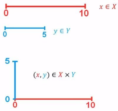
Caso Certero
El plano x-y son todos los pares posibles entre los números de X y Y
Caso Difuso
\mu_{A \times B}(x,y) = \min ( \mu_A(x), \mu_B(y))\begin{aligned}
A & = \left\{ \frac{0}{0}, \frac{0.1}{40}, \frac{0.5}{80}, \frac{0.8}{100}, \frac{1}{120}, \frac{1}{140} \right\} \text{Alta Velocidad} \\
B & = \left\{ \frac{0.8}{1}, \frac{0.8}{2}, \frac{0.9}{3}, \frac{1}{4} \right\} \text{Gravedad del Accidente} \\
\end{aligned} \\
\mathcal{R} = A \times B = \begin{matrix}
\begin{matrix} 0 \\ 40 \\ 80 \\ 100 \\ 120 \\ 140 \end{matrix} & \begin{bmatrix}
0 & 0 & 0 & 0 \\
0.1 & 0.1 & 0.1 & 0.1 \\
0.5 & 0.5 & 0.5 & 0.5 \\
0.8 & 0.8 & 0.8 & 0.8 \\
0.8 & 0.8 & 0.9 & 1.0 \\
0.8 & 0.8 & 0.9 & 1.0 \\
\end{bmatrix} \\
& \begin{matrix} 1 & 2 & 3 & 4 \end{matrix}
\end{matrix}Puede servir para relacionar causa – efecto.
Composición entre Relaciones Difusas
Composición de Funciones Certeras
z = f(y) = f( g(x) ) =: f \circ g (x)
Composición de Relaciones Difusas
Composición Max-Min
\begin{aligned}

\mu_{ \mathcal{R}_1 \circ \mathcal{R}_2 }

& = \lor_y \left[  \mu_{\mathcal{R}_1} (x,y) \land \mu_{\mathcal{R}_2} (y,z) \right] \\

& = \max_y \left\{ \min\left[ \mu_{\mathcal{R}_1} (x,y) , \mu_{\mathcal{R}_2} (y,z) \right] \right\}

\end{aligned}
Composición Max-Producto
\begin{aligned}

\mu_{ \mathcal{R}_1 \circ \mathcal{R}_2 }

& = \max_y \left\{ \mu_{\mathcal{R}_1} (x,y) \mu_{\mathcal{R}_2} (y,z)\right\}

\end{aligned}
Procedimiento de composición (caso max-min):
\begin{aligned}

\mathcal{R}_1 = & A_m \times B_n =  \left[ \mu_{A \times B} (x,y) \right]_{m \times n} = \left[ \min ( \mu_A(x), \mu_B(y) \right]_{m \times n} \to \left[ \mu_{ \mathcal{R}_1}(x,y) \right]_{m \times n} \\

\mathcal{R}_2 = & B_n \times C_p =  \left[ \mu_{B \times C} (y,z) \right]_{n \times p} = \left[ \min ( \mu_B(y), \mu_B(z) \right]_{n \times p} \to  \left[ \mu_{ \mathcal{R}_2 }(y,z) \right]_{n \times p} \\

\mathcal{R}_1 \circ \mathcal{R}_2 = & \left[
\max_y \left\{
\min \left[
\mu_{\mathcal{R}_1}(x,y),
\mu_{ \mathcal{R}_2}(y,z)
\right]
\right\}
\right]_{m \times p} \to \left[ \mu_{\mathcal{R}_1 \circ \mathcal{R}_2} (x,z) \right]_{m \times p} \\

& \text{el elemento } i, j \text{ se determina por:} \\

\left[ \mathcal{R}_1 \circ \mathcal{R}_2 \right]_{i,j} = &
\max \{ \\
& \min \left[
\left[ \mu_{\mathcal{R}_1}(x,y) \right]_{i,1} ,
\left[ \mu_{ \mathcal{R}_2}(y,z) \right]_{1,j}
\right] , \\
& \min \left[
\left[ \mu_{\mathcal{R}_1}(x,y) \right]_{i,2} ,
\left[ \mu_{ \mathcal{R}_2}(y,z) \right]_{2,j}
\right] , \\
& \dots , \\
& \min \left[
\left[ \mu_{\mathcal{R}_1}(x,y) \right]_{i,n-1} ,
\left[ \mu_{ \mathcal{R}_2}(y,z) \right]_{n-1,j}
\right] , \\
& \min \left[
\left[ \mu_{\mathcal{R}_1}(x,y) \right]_{i,n} ,
\left[ \mu_{ \mathcal{R}_2}(y,z) \right]_{n,j}
\right] \\
& \}

\end{aligned}
\begin{aligned}
\mathcal{R}_1 = A \times B & = \begin{bmatrix}
0.4 & 1 & 0.2 \\
0.1 & 0 & 0.5 \\
0.9 & 0.7 & 0.8
\end{bmatrix} \\
\mathcal{R}_2 = B \times C & = \begin{bmatrix}
1 & 0.6 & 0.5 & 0.4 & 0.0 \\
0.4 & 0.8 & 0.7 & 0.3 & 0.3 \\
0.5 & 1.0 & 0.5 & 0.2 & 0.8
\end{bmatrix} \\
\mathcal{R}_1 \circ \mathcal{R}_2 & = \begin{bmatrix}
0.4 & 1 & 0.2 \\
0.1 & 0 & 0.5 \\
0.9 & 0.7 & 0.8
\end{bmatrix} \begin{bmatrix}
1 & 0.6 & 0.5 & 0.4 & 0.0 \\
0.4 & 0.8 & 0.7 & 0.3 & 0.3 \\
0.5 & 1.0 & 0.5 & 0.2 & 0.8
\end{bmatrix} \\
& = \begin{bmatrix}
0.4 & 0.8 & 0.7 &0.4 & 0.3 \\
0.5 & 0.5 & 0.5 & 0.2 & 0.5 \\
0.9 & 0.8 & 0.7 & 0.4 & 0.8
\end{bmatrix}
\end{aligned}\begin{aligned}
(\mathcal{R}_1 \circ \mathcal{R}_2)_{1,1}
& = \max \left\{
\min \left[ (\mathcal{R}_1)_{1,1} , (\mathcal{R}_2)_{1,1} \right],
\min \left[ (\mathcal{R}_1)_{1,2} , (\mathcal{R}_2)_{2,1} \right],
\min \left[ (\mathcal{R}_1)_{1,3} , (\mathcal{R}_2)_{3,1} \right],
\right\} \\
& = \max \left\{
\min \left[ 0.4 , 1 \right],
\min \left[ 1 , 0.4 \right],
\min \left[ 0.2, 0.5 \right],
\right\} \\
& = \max \left\{
0.4,
0.4,
0.2,
\right\} \\
& = 0.4 \\
(\mathcal{R}_1 \circ \mathcal{R}_2)_{2,4}
& = \max \left\{
\min \left[ (\mathcal{R}_1)_{2,1} , (\mathcal{R}_2)_{1,4} \right],
\min \left[ (\mathcal{R}_1)_{2,2} , (\mathcal{R}_2)_{2,4} \right],
\min \left[ (\mathcal{R}_1)_{2,3} , (\mathcal{R}_2)_{3,4} \right],
\right\} \\
& = \max \left\{
\min \left[ 0.1 , 0.4 \right],
\min \left[ 0.0 , 0.3 \right],
\min \left[ 0.5, 0.2 \right],
\right\} \\
& = \max \left\{
0.1,
0.0,
0.2,
\right\} \\
& = 0.2
\end{aligned}[Hackeando Tec]. (2015, Agosto ). Lógica Difusa – 2.1.1 Relaciones Difusas – Hackeando Tec [Video]. YouTube. https://youtu.be/GDXDlTsXF1c?si=wQSPLnaMbM5zWoSP
[Hackeando Tec]. (2015, Agosto ). Lógica Difusa – 2.1.2 Producto Cartesiano Difuso – Hackeando Tec [Video]. YouTube. https://youtu.be/Xki34v7gIug?si=LY2zWzfuDjeWm1WF
[Hackeando Tec]. (2015, Agosto ). Lógica Difusa – 2.1.3 Composición entre relaciones difusas – Hackeando Tec [Video]. YouTube. https://youtu.be/Q13I0JzJ2lo?si=BiI6UxW5Zs7T6dRn